

Prerequisites
The metrics are available in the Explore section of the Grafana instance that CoreWeave hosts. To access Grafana, you must be logged into the CoreWeave Cloud Console and be a member of theadmin, metrics, or write groups.
To open the Explore view, follow these steps:
- Log into the CoreWeave Cloud Console.
- Click Grafana in the left-hand navigation menu.
- Within Grafana, select Explore in the left-hand navigation menu.
Key usage metrics
These metrics provide insight into resource consumption. You can query them directly to create time-series graphs or compute aggregations. The sections that follow describe the metrics available for compute, storage, and networking, along with the labels you can use to filter and group results.Compute usage
Metric billing:instance:total
This metric provides the number of Nodes (instances) running in the selected clusters. Units are in instances.
These labels are available for filtering and grouping:
Clusters created before July 7, 2025 should filter out the
cpu-control-plane Node Pool with the following query when estimating billable compute usage:node_pool_name != "cpu-control-plane"These Nodes aren’t billable. Clusters created after this date don’t have a cpu-control-plane Node Pool.Storage usage
Metric billing:object_storage_used_bytes:total
This metric provides the amount of data stored in CoreWeave AI Object Storage. Units are in bytes.
The following labels are available for filtering and grouping:
CoreWeave only guarantees that the underlying data for this metric updates once per hour.
Metric billing_resource_usage_storage
This metric provides the size of storage volumes provisioned for CKS clusters. Units are in bytes.
The following labels are available for filtering and grouping:
Networking usage
Metric billing_ip_address
This metric provides the number of public IP addresses provisioned in your CKS clusters. These are typically associated with LoadBalancer Kubernetes services. Units are in public IP addresses.
The following labels are available for filtering and grouping:
Practical monitoring examples
The following scenarios show how to combine the metrics above into queries that answer common questions about usage and cost.Explore usage trends over time
Visualizing usage trends helps you spot patterns, detect anomalies, and assess the impact of changes. Long-term trends can support forecasting, and short-term trends can reveal issues. To explore usage trends, follow these steps:- Navigate to Grafana’s Explore section. See Prerequisites.
- Select a desired Time range using the picker in the top right.

- Enter your query in the query editor.

- Ensure the query Type in the Options section is set to Range or Both.
- Click Run query, or press Shift+Enter.
Example: Billable GPU and CPU instances grouped by type
Use this query to find the count of billable instances, grouped by their type.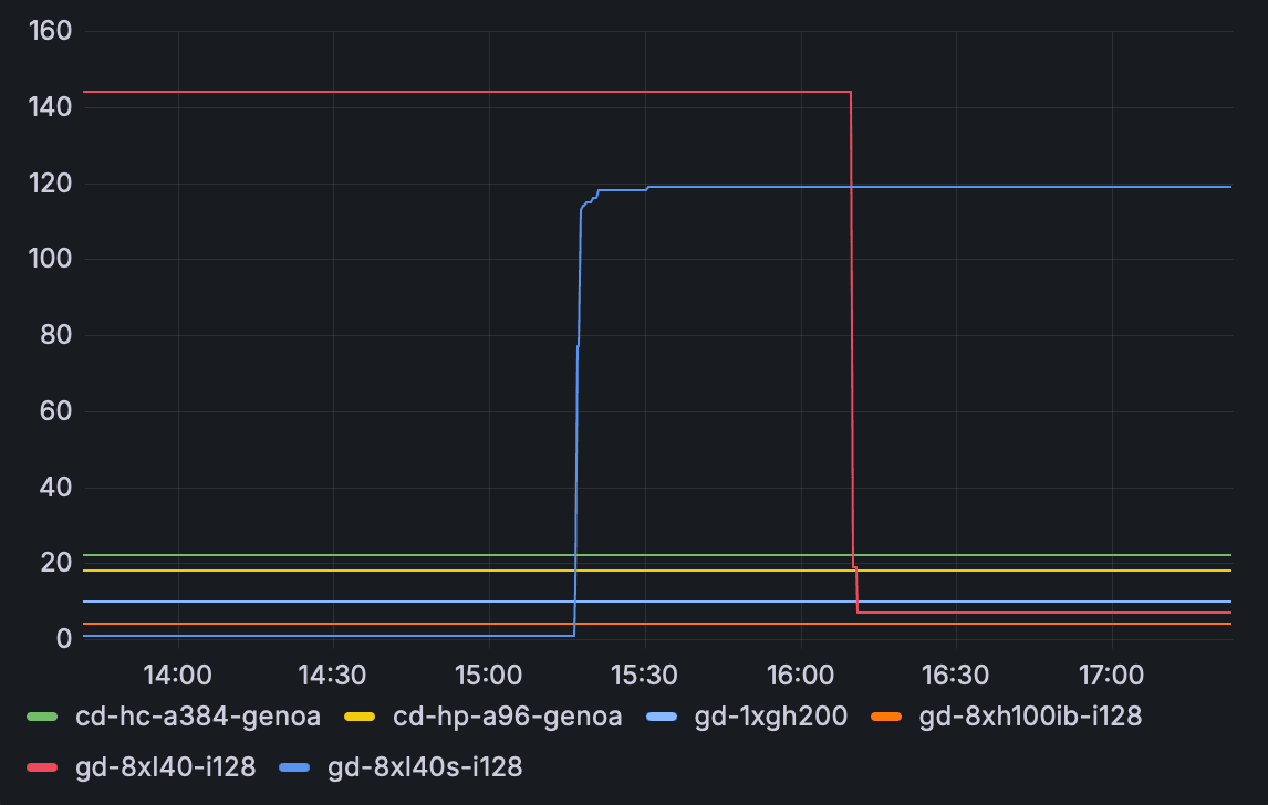
Example: Billable AI Object Storage grouped by bucket in GiB
Use this query to find the total storage used in CoreWeave AI Object Storage, grouped by bucket name and converted to GiB.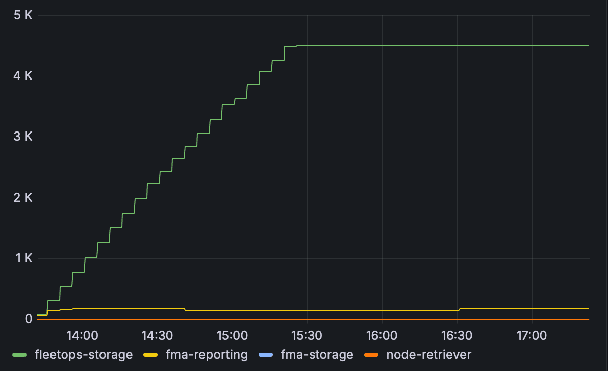
Example: Distributed File Storage in GiB
Use this query to find the total provisioned size of storage volumes that use the shared-vast storage class, converted to GiB.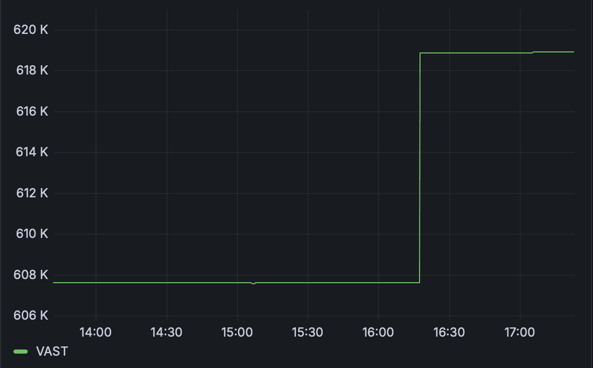
Estimate total On-Demand costs for a time period
While Reserved instances provide guaranteed access at a fixed rate, any usage beyond Reservations is metered as On-Demand. You can estimate your On-Demand costs using Grafana, which helps with forecasting spend or reconciling expected charges before the billing cycle closes.This provides an estimate based on standard On-Demand rates and your real-time usage metrics. Actual billed amounts can vary based on contracts, discounts, taxes, and billing cycle specifics.
Example: Month-to-date On-Demand estimate excluding Reservation
Assume the following scenario:- 25 Reserved H200 Nodes (
gd-8xh200ib-i128). - L40S Nodes run On-Demand (
gd-8xl40s-i128). - General Purpose AMD Genoa Nodes run On-Demand (
cd-gp-a192-genoa). - Object Storage, Distributed Filesystem Storage, and Public IP addresses are in use.
- No additional discounts on On-Demand usage.
- Navigate to Grafana’s Explore section. See Prerequisites.
- Select This month so far in the time range picker.
-
Enter the following query, replacing the instance types and prices with your specific details and current On-Demand rates:
- Ensure the query Type in the Options section is set to Instant.
- Click Run query, or press Shift+Enter.
About range vectors and step size
In this query,$__range:30s sets the time range and the step size for the data. The 30s step means the query evaluates data points every 30 seconds across the selected time range in Grafana.
The query uses a divisor of 120 to normalize the total across all 30-second intervals in a 1-hour range. This converts the result into an average hourly rate. For example, one hour contains 120 intervals when using a 30-second step: 60 minutes multiplied by 2.
If you change the step size, update the divisor to match. For example:
- Use
60for a1mstep size. - Use
240for a15sstep size.
Assess GPU utilization
Monitoring GPU utilization helps determine if you’re using your GPU resources effectively. High utilization might indicate a need for more capacity or Reservations, and low utilization could suggest opportunities for scaling down or consolidating workloads.Example: Average H100 GPU utilization, including SUNK and non-SUNK workloads
This query calculates the average utilization percentage for H100 GPUs over the selected time range. It considers both GPUs that SUNK jobs allocate and GPUs that other workloads use, excluding specific verification namespaces. To assess the average GPU utilization for H100 GPUs, follow these steps:- Navigate to Grafana’s Explore section. See Prerequisites.
- Select your desired Time range.
-
Enter the following query:
- Ensure the query Type in the Options section is set to Instant.
- Click Run query, or press Shift+Enter.
label_node_kubernetes_io_instance_type, label_gpu_nvidia_com_model, and GPUs-per-node multiplier, for example * 8, according to the specific instance types you’re analyzing.