Smooth line plots - CoreWeave Docs

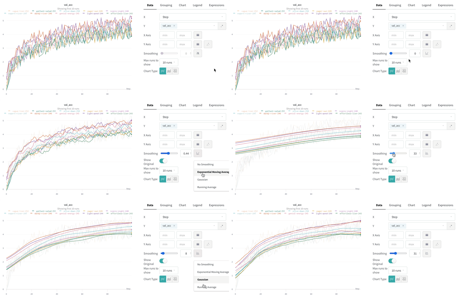
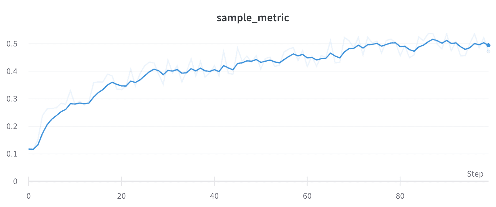
Smoothing helps you spot trends in noisy line plots by reducing point-to-point variation, making the underlying signal easier to read. This page describes the smoothing algorithms Weights & Biases supports, when each one is most useful, and how to control whether the original data remains visible. Weights & Biases supports several types of smoothing:

Time weighted exponential moving average (TWEMA) smoothing
Gaussian smoothing
Running average
Exponential moving average (EMA) smoothing

To see these algorithms applied to real data, see this interactive W&B report.

Comparison of various smoothing algorithms applied to a noisy line plot

Time weighted exponential moving average (TWEMA) smoothing (default)

The time-weighted exponential moving average (TWEMA) smoothing algorithm is a technique for smoothing time series data by exponentially decaying the weight of previous points. For details about the technique, see Exponential Smoothing. The range is 0 to 1. A debias term is added so that early values in the time series aren’t biased towards zero. The TWEMA algorithm takes the density of points on the line (the number of y values per unit of range on x-axis) into account. This allows consistent smoothing when displaying multiple lines with different characteristics simultaneously. The following sample code shows how this works under the hood:

const smoothingWeight = Math.min(Math.sqrt(smoothingParam || 0), 0.999);
let lastY = yValues.length > 0 ? 0 : NaN;
let debiasWeight = 0;

return yValues.map((yPoint, index) => {
  const prevX = index > 0 ? index - 1 : 0;
  // VIEWPORT_SCALE scales the result to the chart's x-axis range
  const changeInX =
    ((xValues[index] - xValues[prevX]) / rangeOfX) * VIEWPORT_SCALE;
  const smoothingWeightAdj = Math.pow(smoothingWeight, changeInX);

  lastY = lastY * smoothingWeightAdj + yPoint;
  debiasWeight = debiasWeight * smoothingWeightAdj + 1;
  return lastY / debiasWeight;
});

To see this algorithm applied to live data, see the TWEMA section of the interactive W&B report.

Gaussian smoothing

Gaussian smoothing (or Gaussian kernel smoothing) computes a weighted average of the points, where the weights correspond to a Gaussian distribution with the standard deviation specified as the smoothing parameter. Weights & Biases calculates the smoothed value for every input x value, based on the points that occur both before and after it. To see this algorithm applied to live data, see the Gaussian smoothing section of the interactive W&B report.

Running average smoothing

Running average is a smoothing algorithm that replaces a point with the average of points in a window before and after the given x value. See “Boxcar Filter” on Wikipedia. The selected parameter for running average specifies the number of points to consider in the moving average. If your points are spaced unevenly on the x-axis, use Gaussian smoothing instead, because a fixed-width window can produce misleading averages when point density varies. To see this algorithm applied to live data, see the running average section of the interactive W&B report.

Exponential moving average (EMA) smoothing

The exponential moving average (EMA) smoothing algorithm is a heuristic technique for smoothing time series data using the exponential window function. For details about the technique, see Exponential Smoothing. The range is 0 to 1. A debias term is added so that early values in the time series aren’t biased towards zero. In most cases, EMA smoothing applies to a full scan of history, rather than bucketing first before smoothing. This typically produces more accurate smoothing. In the following situations, EMA smoothing is applied after bucketing instead:

Sampling
Grouping
Expressions
Non-monotonic x-axes
Time-based x-axes

The following sample code shows how this works under the hood:

  data.forEach(d => {
    const nextVal = d;
    last = last * smoothingWeight + (1 - smoothingWeight) * nextVal;
    numAccum++;
    debiasWeight = 1.0 - Math.pow(smoothingWeight, numAccum);
    smoothedData.push(last / debiasWeight);

To see this algorithm applied to live data, see the EMA section of the interactive W&B report.

Hide original data

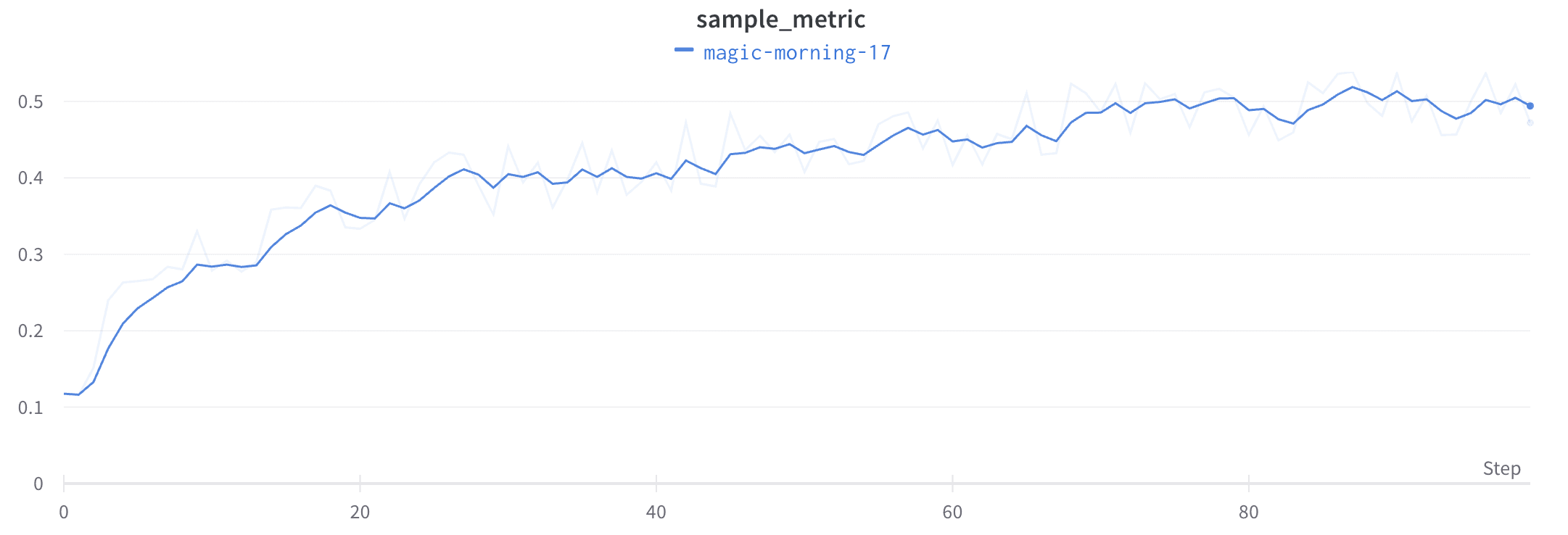
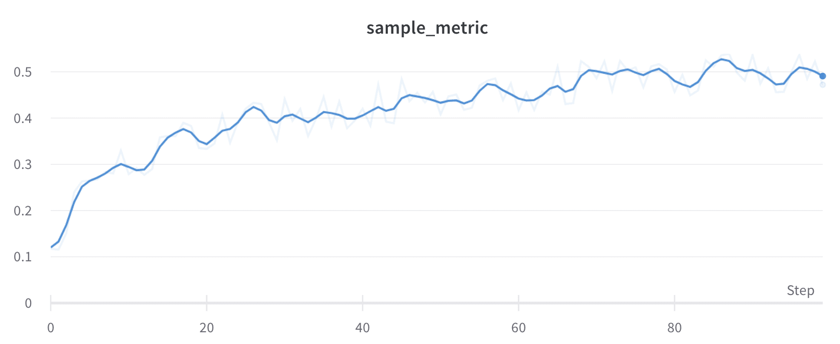
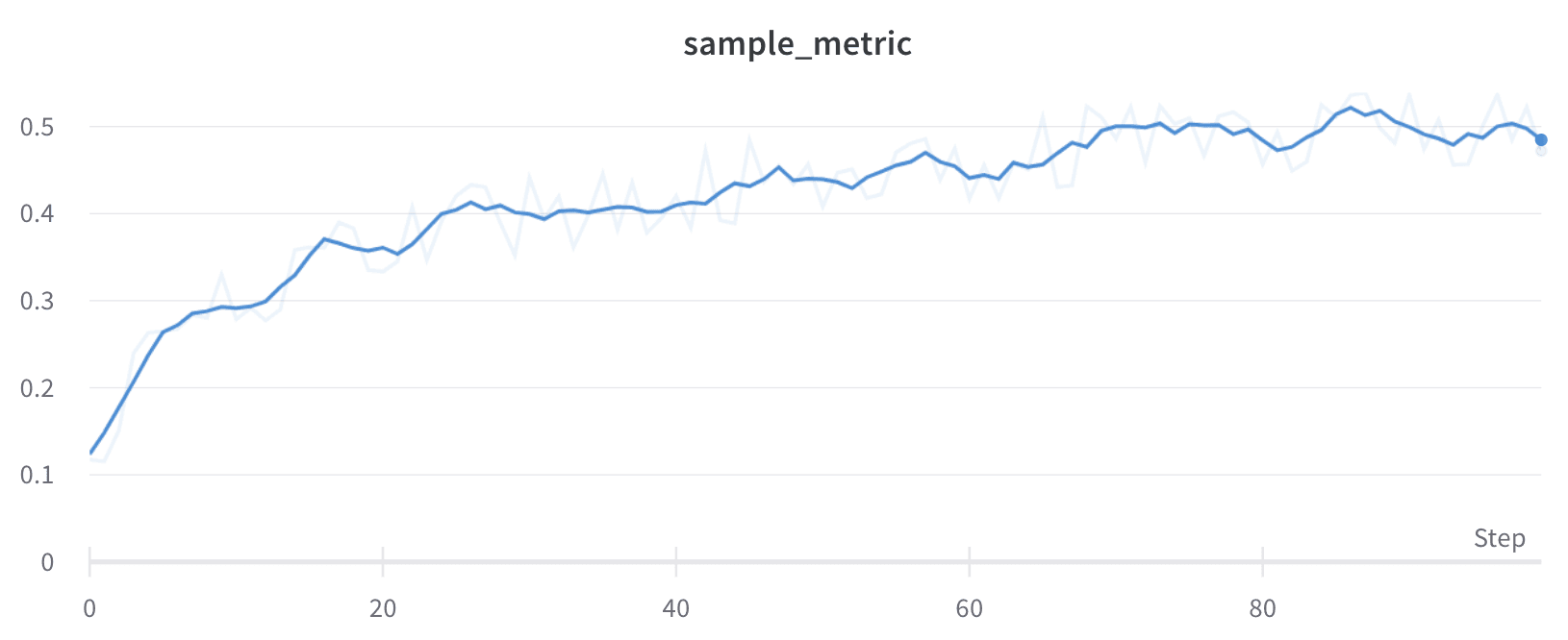
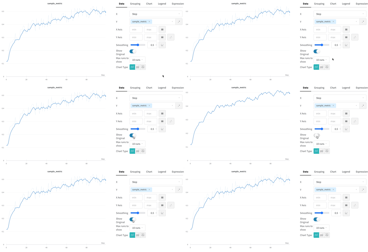
Compare the smoothed line to the raw data to judge how aggressively smoothing alters the signal. By default, the original unsmoothed data displays in the plot as a faint line in the background. Click Show Original to turn this off.

Toggling the display of the original unsmoothed data in a line plot

​Time weighted exponential moving average (TWEMA) smoothing (default)

​Gaussian smoothing

​Running average smoothing

​Exponential moving average (EMA) smoothing

​Hide original data

Time weighted exponential moving average (TWEMA) smoothing (default)

Gaussian smoothing

Running average smoothing

Exponential moving average (EMA) smoothing

Hide original data